Excel bar diagram
There are two main steps in creating a bar and. Select the data you want to visualize.

Bar Chart Inspiration Buscar Con Google Bar Chart Chart Excel
On the Chart Design tab click Add Chart Element point to UpDown Bars and then click Updown Bars.

. Then in the popped out Create Sparklines dialog box. Select the Bar graph since we are going to create a stacked bar chart. Depending on the chart type some options may not be available.
In the beginning you can generate a Stacked Column Chart in Excel and display percentage values by following these steps. Secondly select Format Data Series. First insert all your data into a worksheet.
From the Insert tab select the drop down arrow next to Insert Pie or Doughnut Chart. Click on any one. Format Data Series dialog box will appear on the right side of the screen.
You should find this in the Charts group. There are actually 4 types of bar graphs available in Excel. Firstly Right-Click on any bar of the stacked bar chart.
Grouped bar graph which shows bars of data for multiple variables. Firstly select the data range that we wish to use for the graph. Secondly go to the Insert tab from the ribbon.
This article assists all levels of Excel users on how to create a bar and line chart. A Multiple Bar Graph in Excel is one of the best-suited visualization designs in comparing within-groups and between-groups comparison insights. Select the Stacked Bar graph from the list.
Simple bar graph which shows bars of data for one variable. Show Percentage in a Stacked Bar Chart. Select the cell containing the data.
Bar and Line Graph. Bar charts are one of the most popular ways to visualize data and Excel makes it easy to create them. Select the cells where you want to insert the progress bars and then click Insert Column in the Sparklines group see screenshot.
To create a bar chart execute the following steps. Select the Insert Tab from the top and select the bar chart. From the dropdown menu that appears select the Bar of Pie.
Bar Chart with Line. To create the overlapping bar chart follow the following steps. Select the range A1B6.
Then select the Charts menu and click More. In our case we select the whole data range B5D10. Click the Insert tab on the.
Use a bar chart if you have large text labels. Below are the two format styles for the stacked bar chart. On the Insert tab in the Charts group click the Column symbol.
Finally select a 2D bar chart from. At first select the data and click the Quick Analysis tool at the right end of the selected area. After that the Insert Chart dialogue.
Here are the steps you need to follow to create a bar chart in Excel. The chart is straightforward and easy to.

Free Budget Vs Actual Chart Excel Template Download Excel Templates Budgeting Excel

Adding Up Down Bars To A Line Chart Chart Excel Bar Chart

Gantt Box Chart Tutorial Template Download And Try Today Chart Gantt Chart Online Tutorials

Conditional Formatting Of Excel Charts Peltier Tech Blog Excel Spreadsheets Excel Bar Graphs
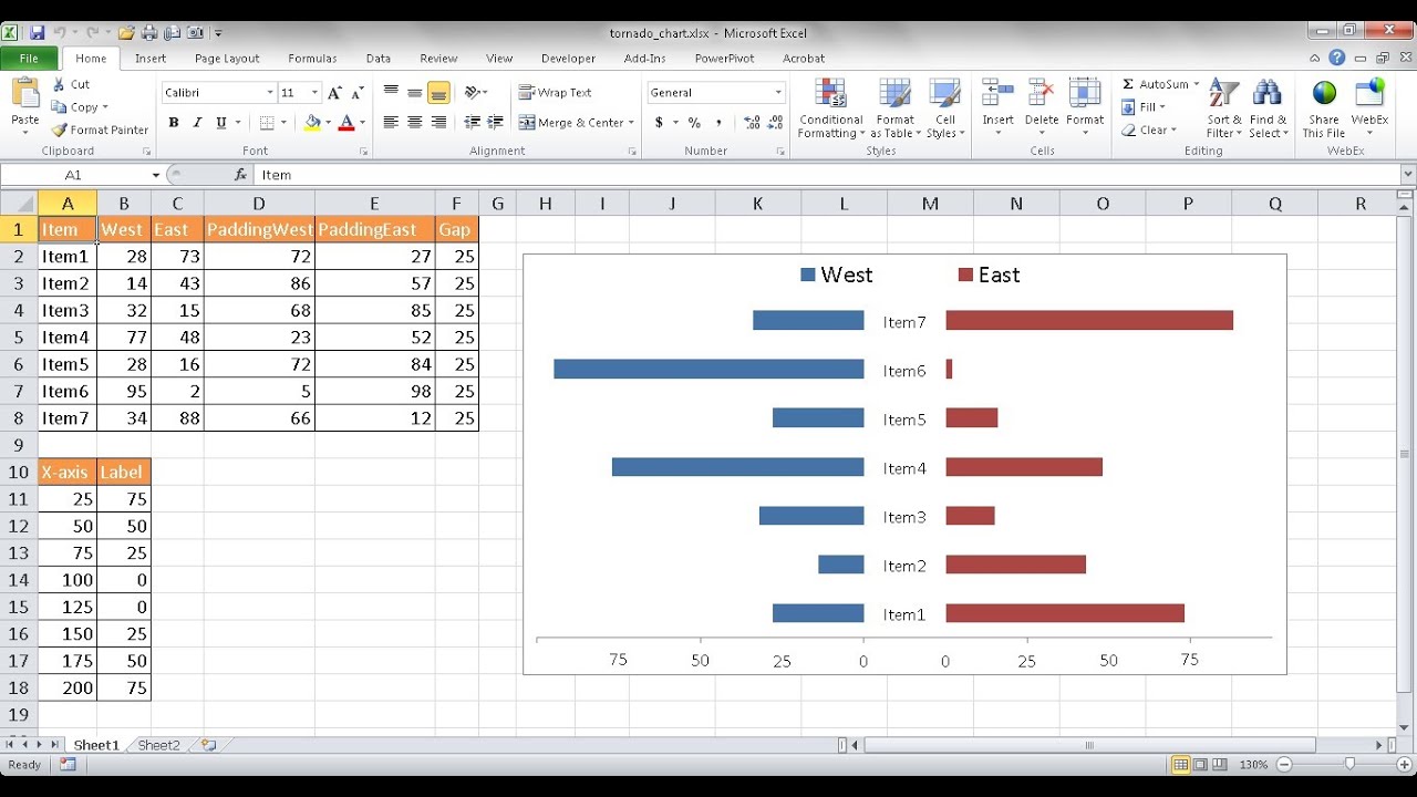
Create A Tornado Butterfly Chart Excel Excel Shortcuts Diagram

Side By Side Bar Chart In Excel Bar Chart Chart Data Visualization

Infographic Pencil Bar Chart In Excel 2016

Excel Chart Elements Element Chart Chart Invoice Format In Excel

Excel How To Create A Dual Axis Chart With Overlapping Bars And A Line Chart Visualisation Excel

How To Build A 2x2 Panel Chart Peltier Tech Blog Chart Data Visualization Information Design

Pin On Microsoft Excel

Pin On Microsoft Excel Charts
Figure 4 Excel Chart Microsoft Excel

Bar Graph Example 2018 Corner Of Chart And Menu Bar Graphs Graphing Diagram

Bar Chart Example Projected International Population Growth Bar Graphs Bar Graph Template Chart

Construction Project Schedule Template Excel Best Of Gantt Chart Charting Bar Pla Excel Templates Excel Templates Project Management Employee Handbook Template

Charts In Excel Excel Tutorials Chart Excel Templates